Getting Started
To get going with EvilPlot, you’ll need to add it to your build. EvilPlot is published for Scala 2.12 and 2.13.
libraryDependencies += "io.github.cibotech" %% "evilplot" % "0.9.0" // Use %%% instead of %% if you're using ScalaJS
Throughout the getting started guide, we’ll assume you’re working either in a Scala REPL or the Ammonite. We publish an additional utility to make using EvilPlot from the REPL easier. To import it, add:
libraryDependencies += "io.github.cibotech" %% "evilplot-repl" % "0.9.0" // Use %%% instead of %% if you're using ScalaJS
to your build.
Our first plot
EvilPlot is all about building larger graphical capabilities out of smaller ones. What this means for you is that making simple plots is easy, and we don’t have to spend a lot of time going over all the features just to get started. So let’s make our first plot, a simple scatter plot with sequential x-values and random y-values. Then we’ll open that plot up in a new window and take a look at it.
import com.cibo.evilplot._
import com.cibo.evilplot.plot._
import com.cibo.evilplot.plot.aesthetics.DefaultTheme._
import com.cibo.evilplot.numeric.Point

val data = Seq.tabulate(100) { i =>
  Point(i.toDouble, scala.util.Random.nextDouble())
}
displayPlot(ScatterPlot(data).render())

There’s a version of this example which renders to an HTML canvas using ScalaJS here
To break it down:
- EvilPlot uses an implicit theming system, which lets you control the appearance of plots wholesale. In this case, we’re just using the built-in one, so we import it.
ScatterPlotreturns aPlotobject, which is a description of how data should be plotted (plot these points as little circles on the screen), with what components (like axes, a background etc.). In this case, we’ve used no components. All we get is points on the screen!render()onPlotreturns aDrawableobject. Think of aDrawableas a fully specified description of a scene.renderitself does not perform any side-effects, it simply constructs a scene given a plot and a size.- Finally,
displayPlotis an additional utility the opens the plot in a new window. You might not use this inside an application, but it’s useful for exploring in the REPL!
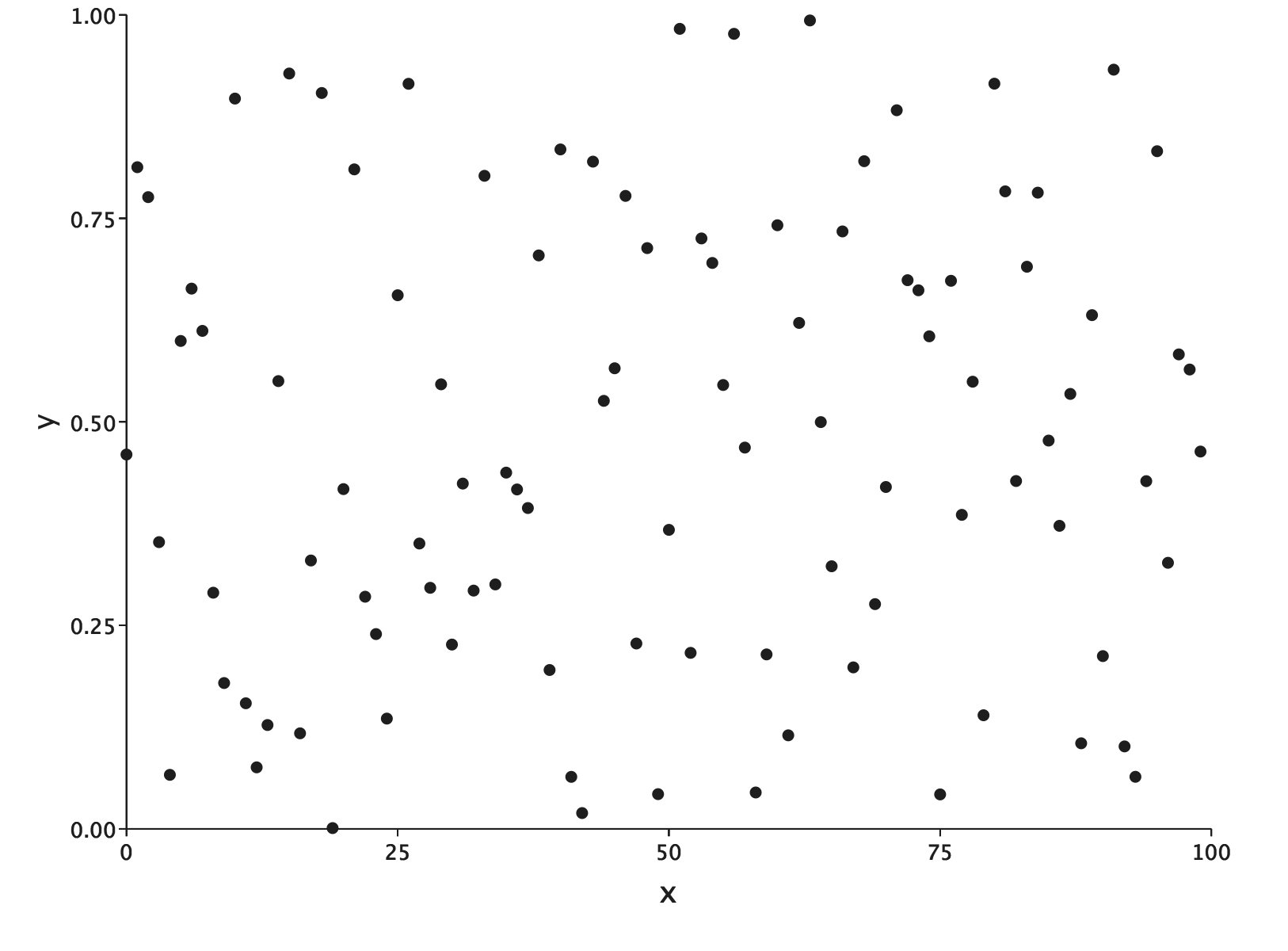
This plot is not very interesting, of course. We should probably add some axes, so we know the range of the data, and some labels, so our audience knows what we’re talking about. That’s easy as well:
import com.cibo.evilplot.plot._
import com.cibo.evilplot.plot.aesthetics.DefaultTheme._
import com.cibo.evilplot.numeric.Point

val data = Seq.tabulate(100) { i =>
  Point(i.toDouble, scala.util.Random.nextDouble())
}
ScatterPlot(data)
  .xAxis()
  .yAxis()
  .frame()
  .xLabel("x")
  .yLabel("y")
  .render()

Adding these things is simply a matter of calling an additional method on your plot that specifies exactly what type of component you want to add.
Plot Construction
Later on we’ll see that EvilPlot actually does not have different types for different kinds of plot – everything is
“just a Plot.” ScatterPlot is just a convenience function that wraps the constructor for Plot. These convenience
functions are likely what you’ll start with most of the time that you use EvilPlot, and there are a bunch of them in the
plot package:
- ScatterPlot
- LinePlot
- ContourPlot
- BoxPlot
- BarChart
- Histogram
- Heatmap
- Facets
- Overlay
Through this tutorial, we’ll see examples of using all of these, but the pattern is mostly the same as what we’ve seen above: call it with your data, add your components, convert to a scene.
The rest of this tutorial is split up as follows:
- Using built-in plots
- A tour of the drawing API.
- How to use plot element renderers, which allow you to fully customize your plots.
- Colors and color utilities